logo
S-Cube is at Transforming Energy Exploration in Bengaluru, India, Sep 23–25!

South LouisianaTSL-FWI™

Highlander · Duck Lake merge · onshore Gulf Coast

The depth at the next well, before the next well

A follow-on exploration problem: one penetration at Highlander 1, a salt canopy, and an Austin Chalk target at 29,000 ft the legacy image could not resolve. Merging three surveys and inverting the minimally-processed field data, to see how far TSL-FWI™ could correct a conventionally-derived existing model with no additional well information.

Austin Chalk target
29,000 ft
From Highlander 1 to the blind tie
3.3 km
Target shift, matched at the well
650 ft
Well investment
$300M
The pipeline
  1. 01

    Data

    Three datasets merged, barely pre-processed.

  2. 02

    Model

    Macro then high-resolution TSL-FWI to 9.5 km.

  3. 03

    Imaging

    Legacy PSDM against RTM on the new model.

  4. 04

    Blind tie

    Highlander 2, drilled after the model shipped.

  5. 05

    Prospect

    The target surface, remapped.

Step 1 · Data

Near-surface prediction, interleaved with the field

Three datasets shot years apart on different geometries, merged and inverted with almost nothing done to them in between. On land the weathering layer distorts every arrival under it, so the near surface is solved first — get it wrong and nothing deeper is worth updating.

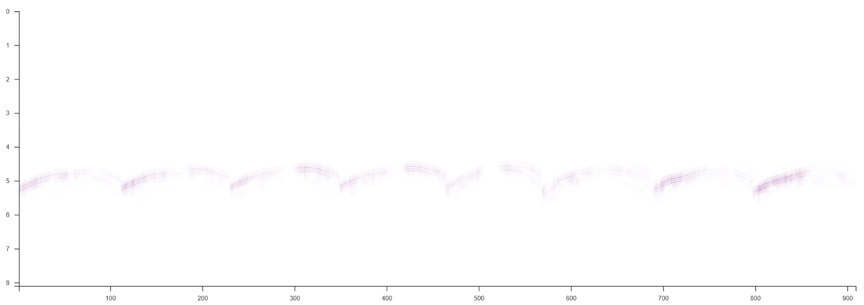
Near surface · shot 1193, interleaved with the field

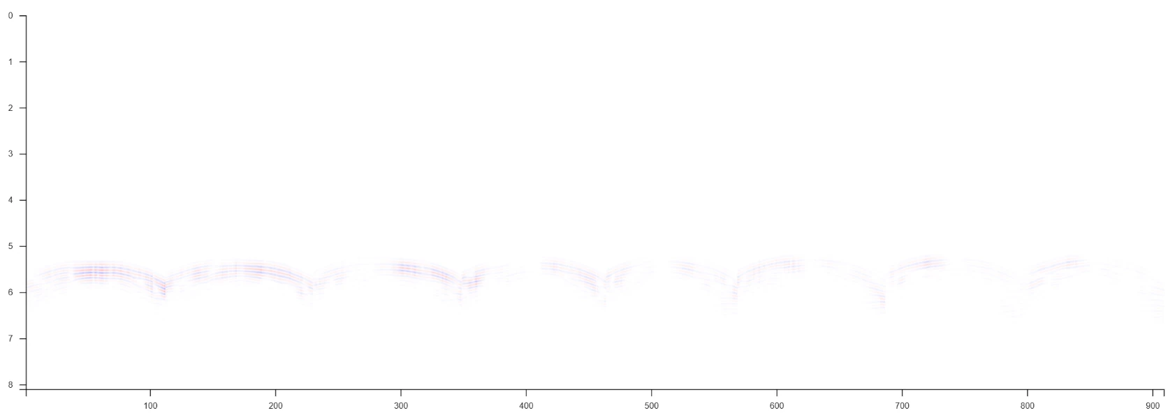
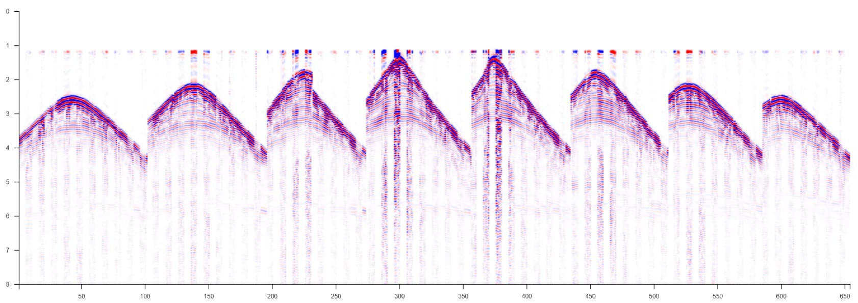
The prediction is spliced into the field record in strips a few traces wide rather than set beside it, because a side-by-side comparison hides small timing errors and this one cannot: where the model is right the events run straight through the seams, where it is wrong they step at every one.
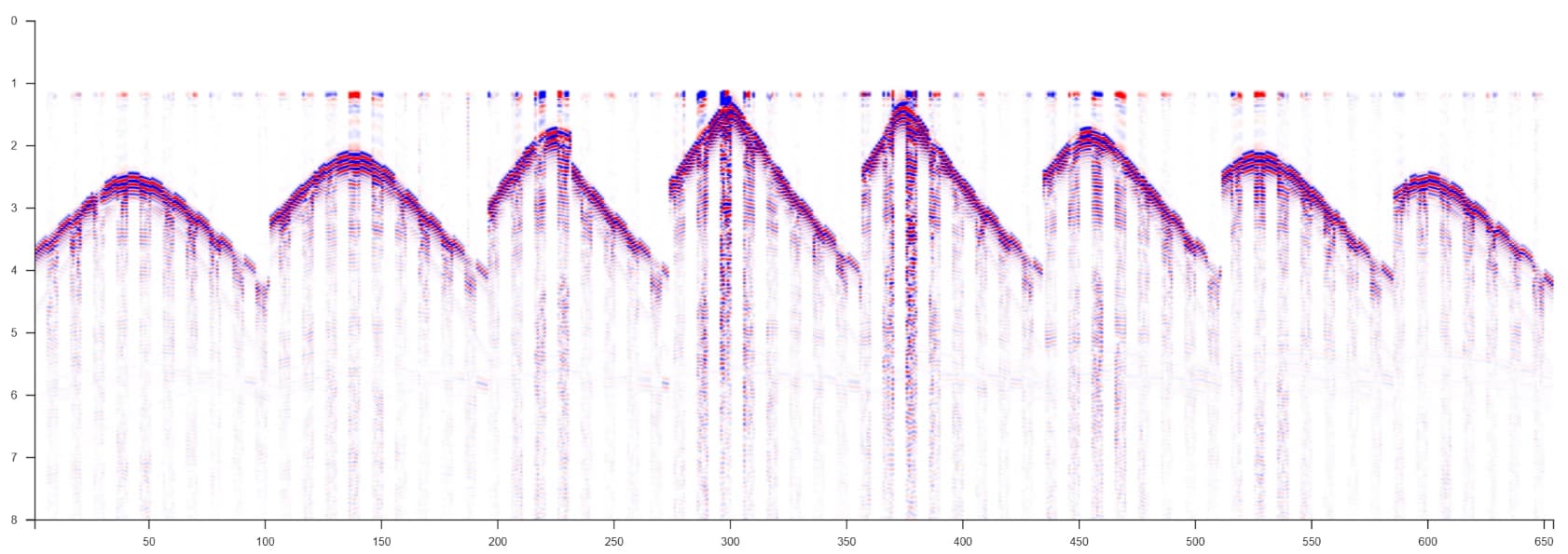
Shot 1193 over eight receiver lines and eight seconds, the starting-model prediction interleaved into the field record, the arrivals patchy and broken
The same interleaved display after the near-surface TSL-FWI update, the arrivals coherent across every fan
1 / 2

The wavetrain breaks into stripes at the seams and the far offsets fall away.

Step 2 · Model

Rebuilding the velocity under the salt

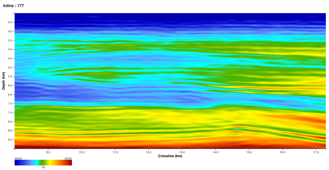
RWI recovers the sub-salt macro trend, then a high-resolution TSL-FWI pass resolves stratigraphy inside it. No horizons picked at any point.

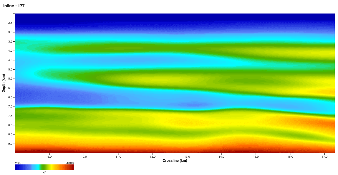
Vp in section · inline 177 & crossline 323
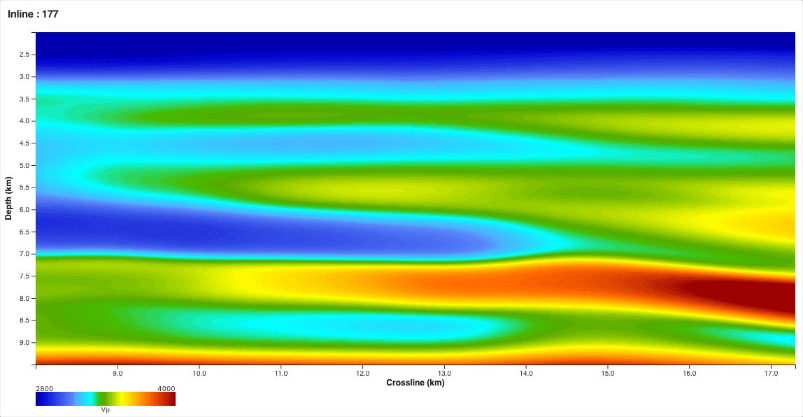
Inline 177 and crossline 323 Vp — the starting velocity model, a smooth layer-cake gradient to 9.5 km
Inline 177 and crossline 323 Vp after the sub-salt macro update from reflection waveform inversion
Inline 177 and crossline 323 Vp after the final high-resolution TSL-FWI pass, resolving stratigraphy at 8.5 to 9 km
1 / 3

A layer-cake gradient. Below 7 km the trend is wrong and nothing separates salt from section.

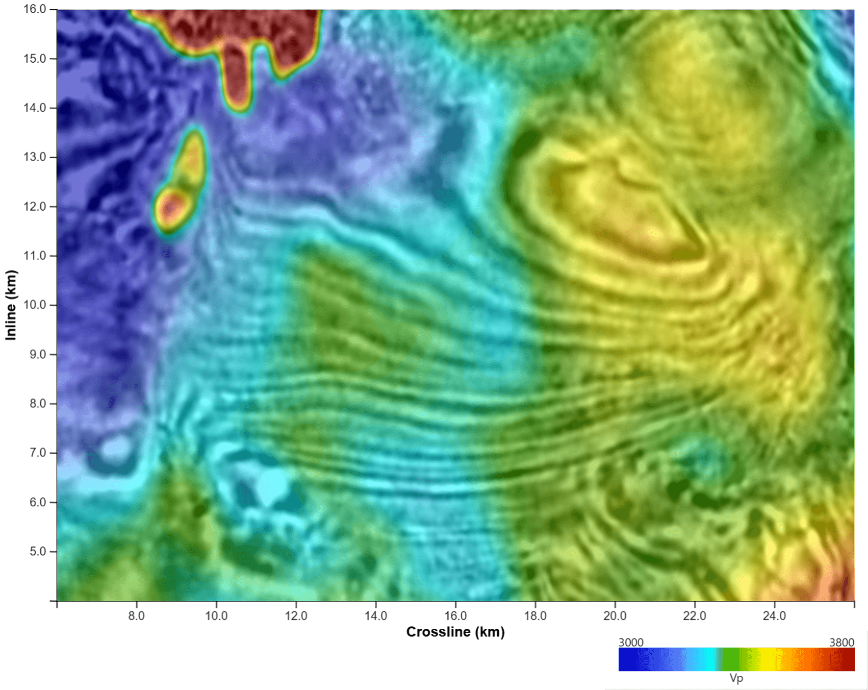
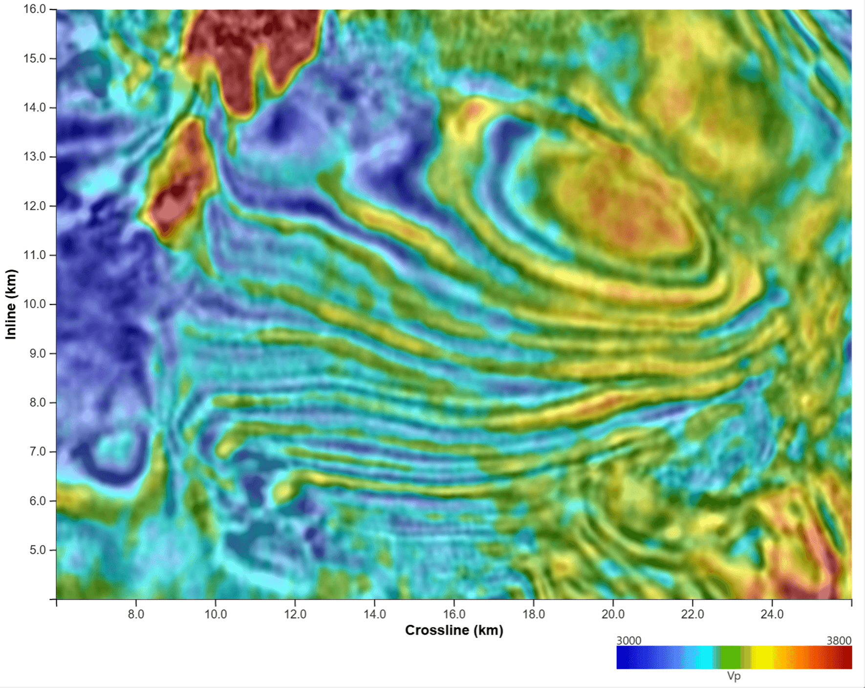
The same model in plan view

Depth slices at 5 km and at 8.3 km — the Austin Chalk level.

Velocity depth slice at 5 km, starting model
Velocity depth slice at 5 km, final TSL-FWI model
1 / 2

A smooth regional gradient — nothing to map at either level.

Step 3 · Imaging

What the new model does to the image

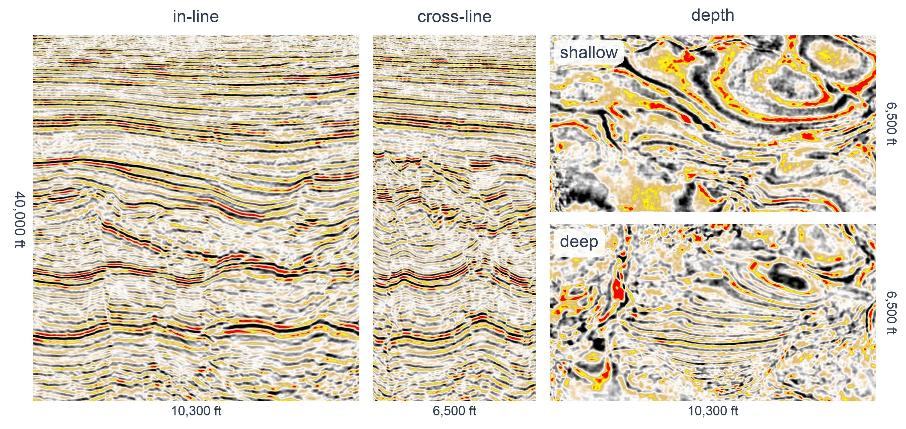
In-line, cross-line and two depth slices, on identical displays. Same data, same migration — only the velocity changed.
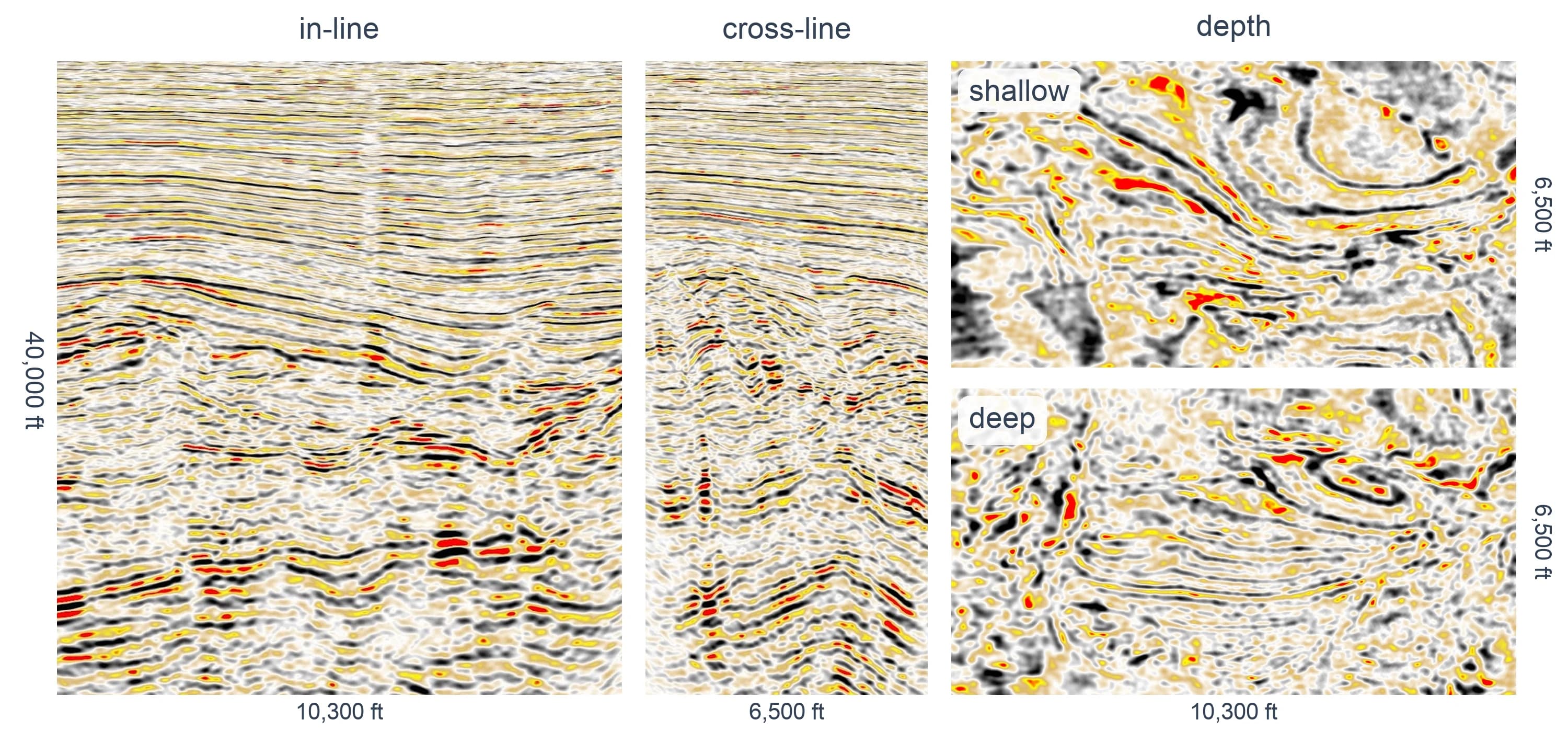
South Louisiana Legacy PSDM: in-line and cross-line sections beside shallow and deep depth slices
South Louisiana RTM · TSL-FWI model: in-line and cross-line sections beside shallow and deep depth slices
1 / 2

The image the prospect was carried on. Broken reflectors below the shallow section; both depth slices closer to noise than structure.

The inversion’s own reflectivity · inline 263 & crossline 216

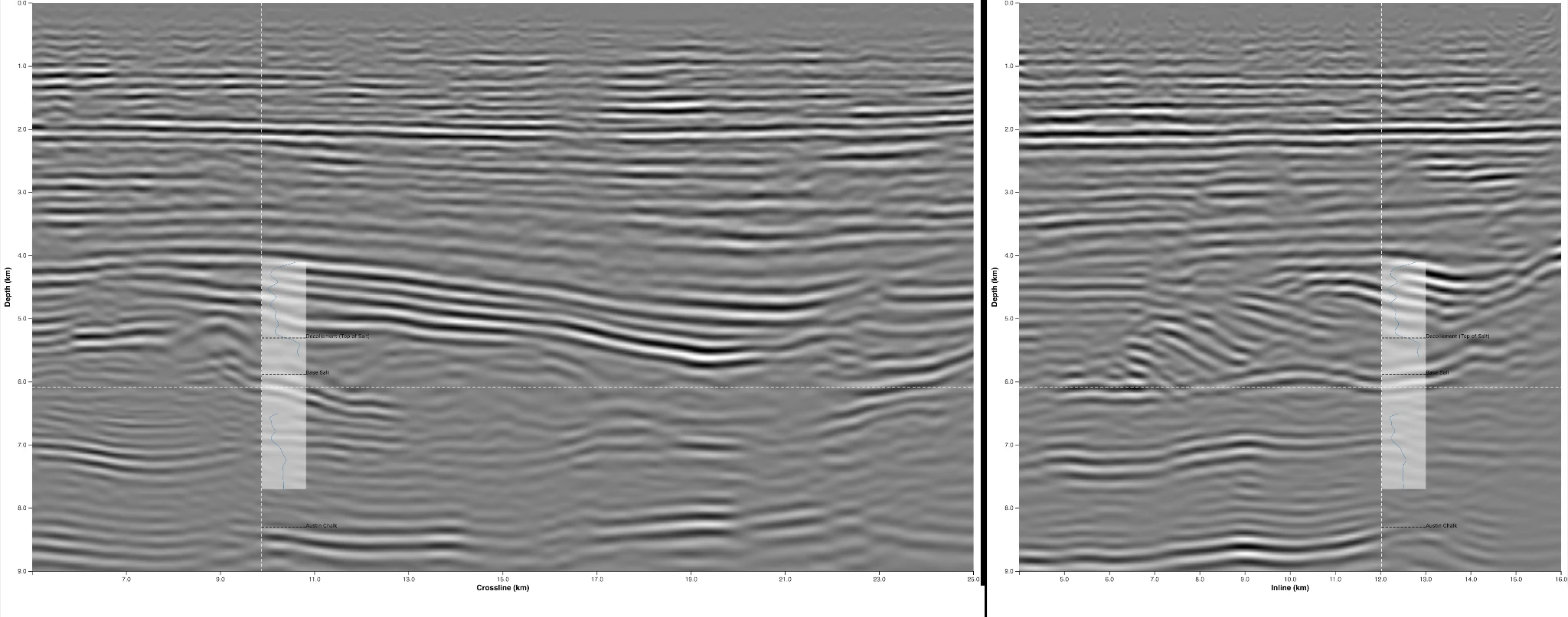
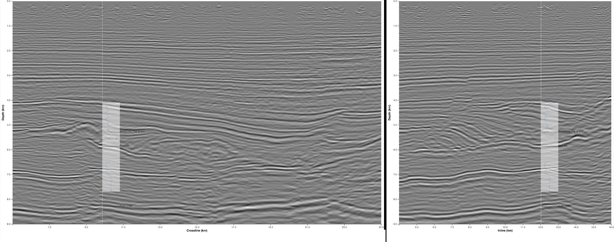
The migration above is not the only image on offer. TSL-FWI solves for density as well as velocity, so it hands back a reflectivity of its own — no migration, no picked velocities, nothing after the inversion. Here it is at 10 Hz and again at 20 Hz: the structure is settled by the first frame and the second fills in the layering, which is what it looks like when the resolution is coming from the data rather than from a migration.

South Louisiana TSL-FWI 10 Hz reflectivity: inline 263 beside crossline 216, zero to 9 km depth, with the decollement, base salt and Austin Chalk picks and the Highlander-1 log annotated
South Louisiana TSL-FWI 20 Hz reflectivity: inline 263 beside crossline 216, zero to 9 km depth, with the decollement, base salt and Austin Chalk picks and the Highlander-1 log annotated
1 / 2

The density contrast the inversion resolved on its own at 10 Hz, displayed as reflectivity. The salt, the decollement and the Austin Chalk are all already there.

Validation · Data fit

The model predicts the recorded shots

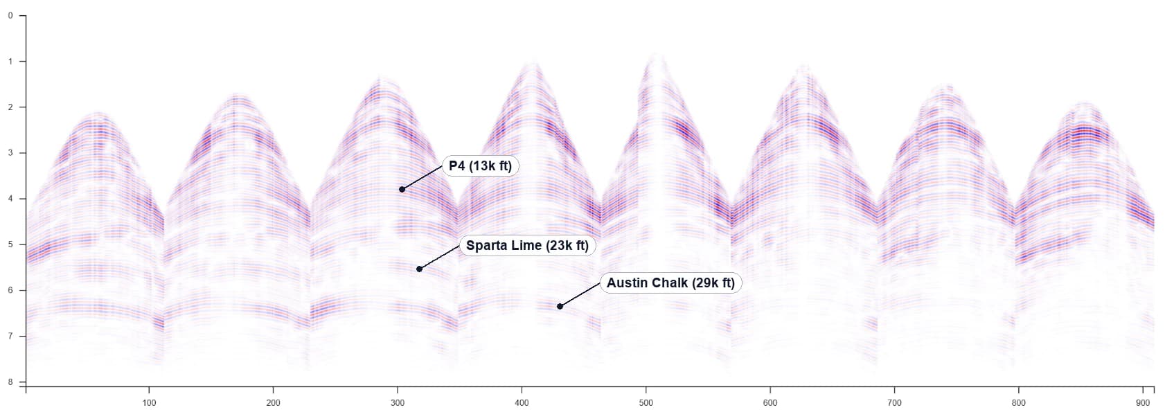
Field gathers against the wavefield modelled through the final model. Not a blind test — the well tie below is that — but it is where the model has to explain the recording event by event.

Shot 1044 · one shot, its receiver lines side by side
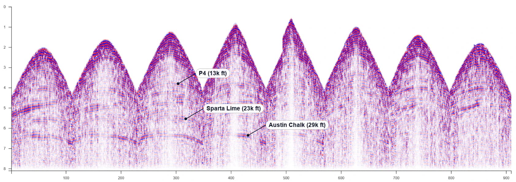
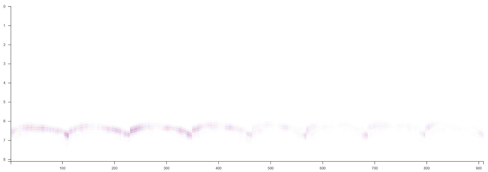
Each fan is one receiver line, so the apex time rises with the line’s distance from the shot. The last three frames are the same prediction with one reflector left in.

Field shot gather 1044, eight receiver-line fans over 900 traces and eight seconds, with the P4, Sparta Lime and Austin Chalk reflections labelled
The same shot modelled through the final TSL-FWI model, with the same three reflections labelled at the same times
The modelled shot with only the base salt reflection left in, arriving just under five seconds
The modelled shot with only the Sparta Lime reflection left in, arriving around five and a half seconds
The modelled shot with only the Austin Chalk reflection left in, arriving just over six and a quarter seconds
1 / 5

The recording. Eight receiver lines, zero to eight seconds.

Validation · Well ties

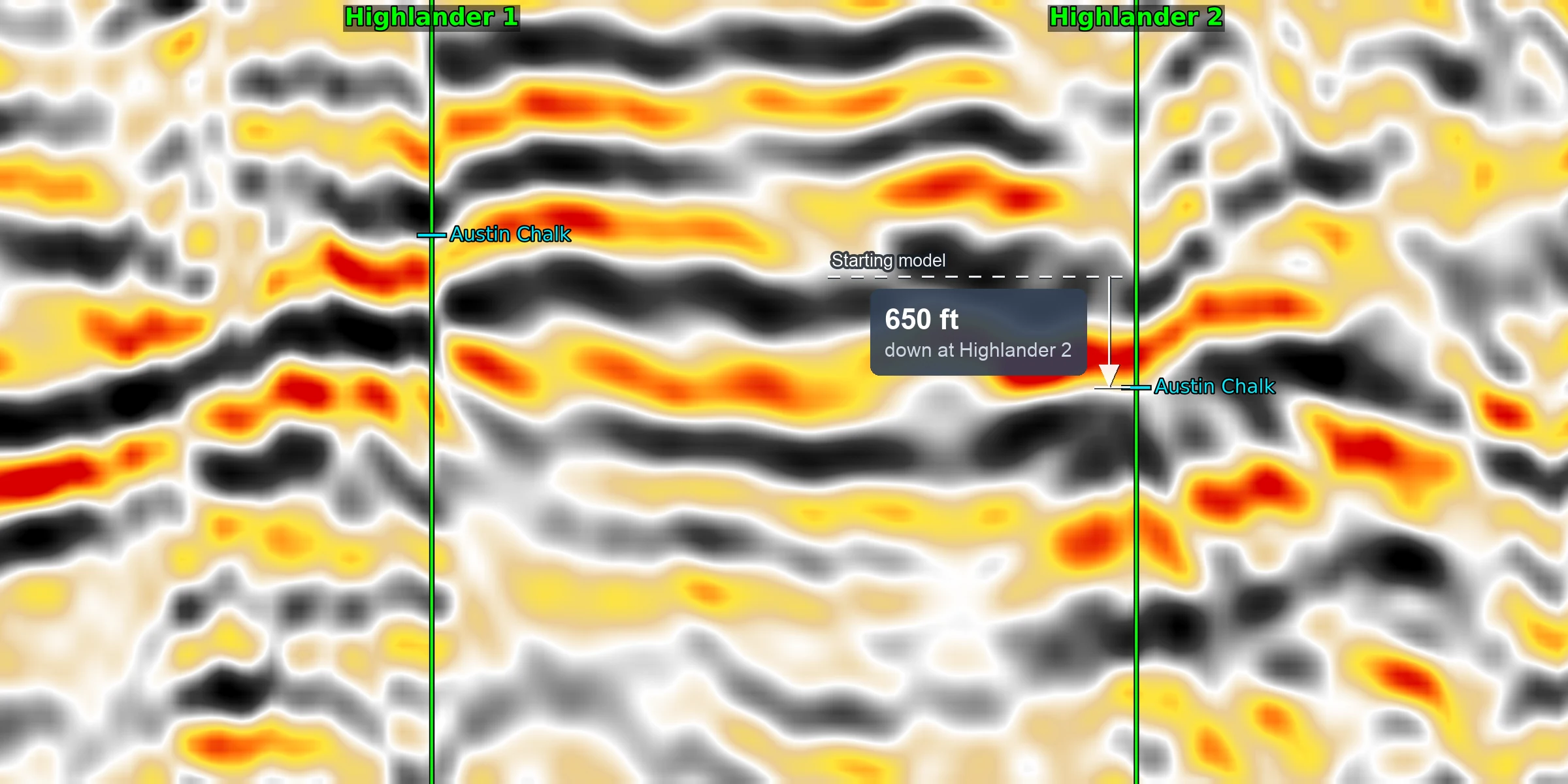
TSL-FWI shifted the target 650 ft

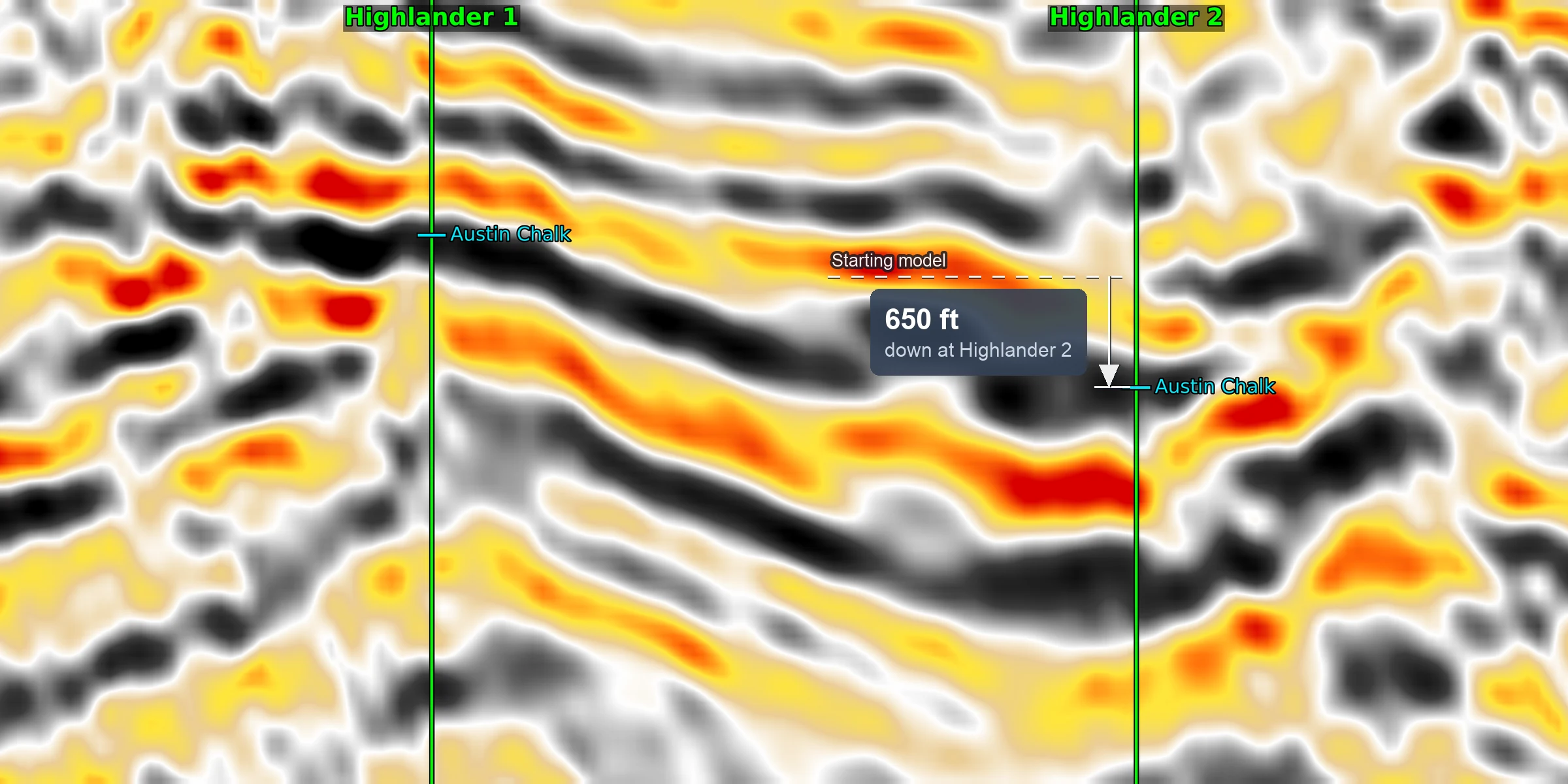
The Austin Chalk moves down 650 ft and comes into focus. Highlander 2, drilled afterwards 3.3 km away, matched it. No wells went into the inversion.

Austin Chalk · target interval, 8.0–9.0 km

RTM through the Austin Chalk interval on the starting model, with the Austin Chalk pick at Highlander 1 and Highlander 2 and the 650 ft the final model moved the chalk down at Highlander 2 marked
RTM through the Austin Chalk interval on the final TSL-FWI model, with the same Austin Chalk picks at Highlander 1 and Highlander 2 and the 650 ft move down at Highlander 2 marked
1 / 2

At Highlander 1 the pick falls in the gap between two events, and at Highlander 2 the chalk sits 650 ft above where the well found it. Between the wells the reflectors wobble and break up.

A purely data-driven velocity correction — free from human bias — that reliably predicts deep structure far from well control.

Four products off one inversion

Everything on this page comes out of one inversion of the merged field data.

Anisotropic TSL-FWI™ velocity

Vp to 9.5 km from the field shots, through the salt to the Austin Chalk. No picked horizons.

RTM on the final model

The operator's own migration, with only the velocity changed.

Like-for-like imaging comparison

Legacy PSDM against the new RTM, on identical displays.

Target surfaces

Austin Chalk and Tuscaloosa remapped on the final volume, before and after.

Step 4 · Prospect

The prospect, mapped

Everything above lands here: the Tuscaloosa sand, remapped on the TSL-FWI volume.
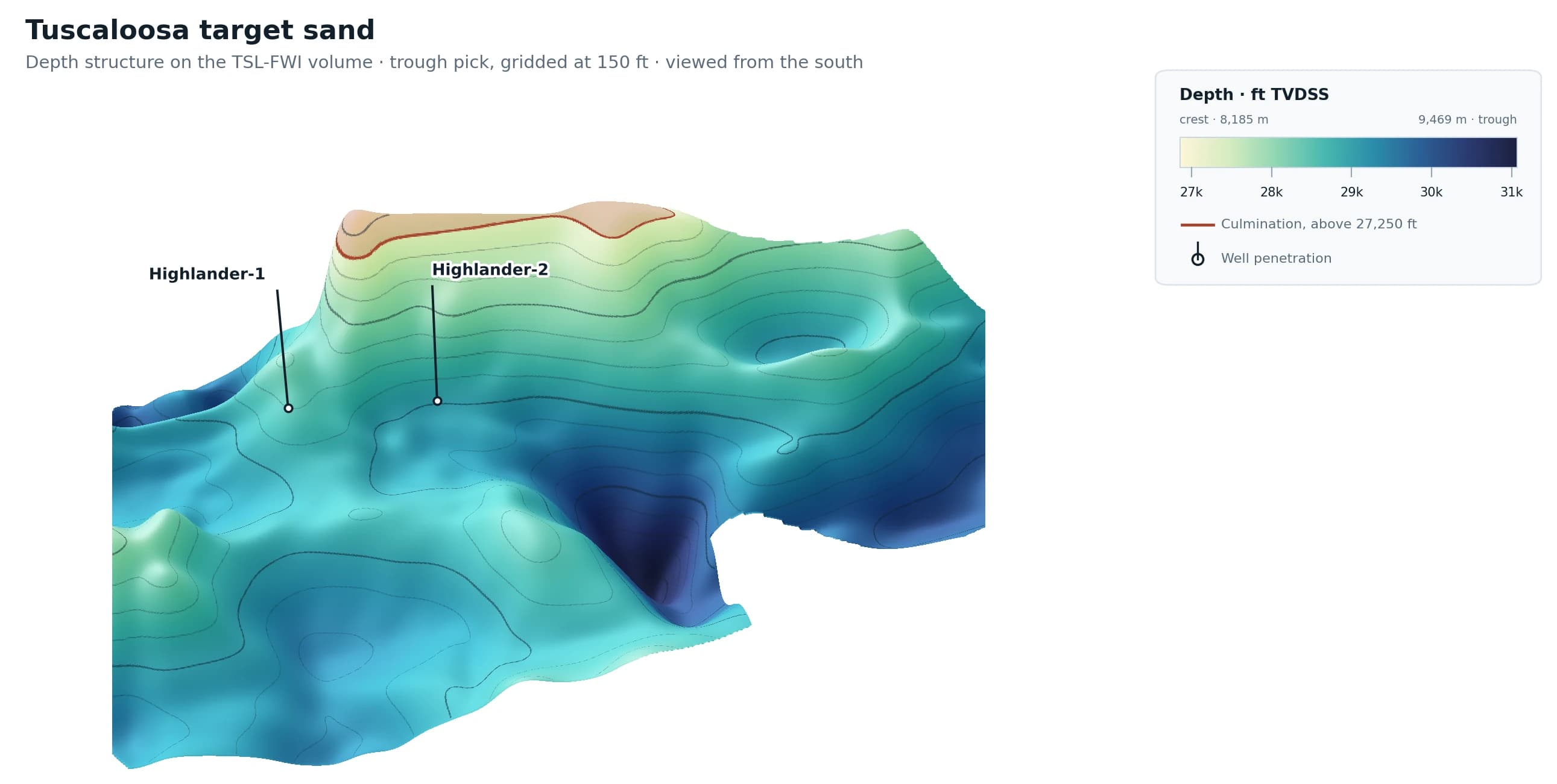
Oblique perspective view of the Tuscaloosa target sand on the TSL-FWI volume, looking north from over the southern edge. The surface covers about 21 by 12 km and runs 26,850 to 31,070 ft TVDSS, contoured every 250 ft under a hypsometric colour ramp, at five times vertical exaggeration. A broad crest stands across the north, tinted and outlined in red where it rises above 27,250 ft; a deep trough cuts through the centre-east and a separate closure sits to the north-east. Highlander-1 and Highlander-2 are marked on stems on the southern flank of the crest, 3.3 km apart, with Highlander-2 the deeper of the two
The sand itself, mapped on the TSL-FWI volume and seen from the south: 26,850–31,070 ft TVDSS, 4,200 ft of relief, a broad crest across the north and a deep trough through the centre. Tinted above 27,250 ft is the crestal culmination — the contours run into the northern limit of the interpretation rather than turning back on themselves, so it is a culmination and not yet a mapped closure. Contours every 250 ft over a 21 × 12 km footprint, at five times vertical exaggeration; the missing south-east corner is the limit of the interpretation, not of the survey.

We can do this on your data

Legacy datasets, minimal pre-processing, no picking — TSL-FWI™ on the field data, back to you in weeks.

Talk to us about your survey

South Louisiana. Three legacy onshore datasets merged and inverted together with X-Wave TSL-FWI™ from the field data. Depths are TVDSS; horizon names and picks are the operator's interpretation.