The data used in this study comes from a field located in the southern North Sea. The depth of the reservoir is approximately 3 km, overlain by an extensive well-confined gas cloud (Granli et al. 1997). The vertical migration of the gas is thought to be the result of piercement of the antiformal structural high caused by an underlying salt diapir. The presence of gas above the reservoir dramatically decreases the quality of the seismic data below; the gas-charged zone has a low p-wave velocity and a high effective attenuation, and both properties appear to degrade the image. Four wells have been drilled on this site: two outside, one at the edge, and one through the gas cloud. Warner et al. (2013), and references therein, provide details.
The data were acquired in 2005. Three swaths of eight ocean-bottom-cables (OBC) were deployed, Figure 1. The cable length was 6 km, the spacing between cables was 300 m, and each contained four-component sensors every 25 m. The source lines were shot perpendicular to the cables using airguns at a depth of 6 m. Dual sources were used in flip-flop shooting mode. Each source consisted of a 3930 cubic inches capacity airgun. The lateral separation between sources was 75 m, and each fired every 50 m in-line. The area covered by each swath was 120 km2 and the three swaths combined covered a total of 180 km2. The total number of four-component receivers in the final dataset is 5760, and the total number of shots is 96,000. The survey provides offsets of around 7 km with good azimuthal coverage, and maximum offsets of up to 11 km with reduced azimuth and fold, corresponding to sources in the corners of the shooting area.
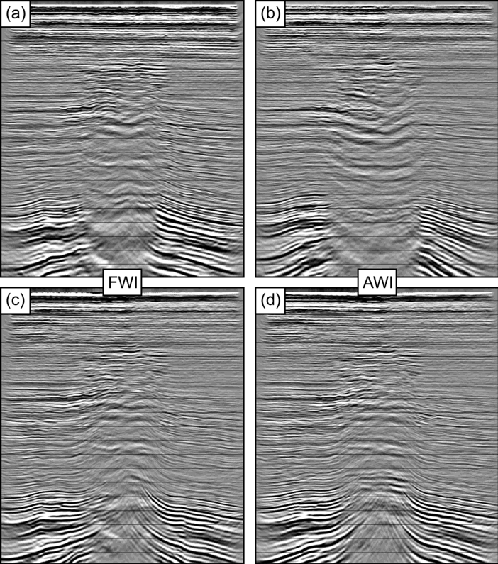
Impact of anomaly on PSDM
Using models with inaccurate / not accounted for low velocity gas zone leads to (1) an obscured zone in the central anticline (2) distorted reflectivity geometry
Much less change from B (tomography) to C (FWI) than A (1d) to D (AWI). In D, reflectors can be best tracked through gas.
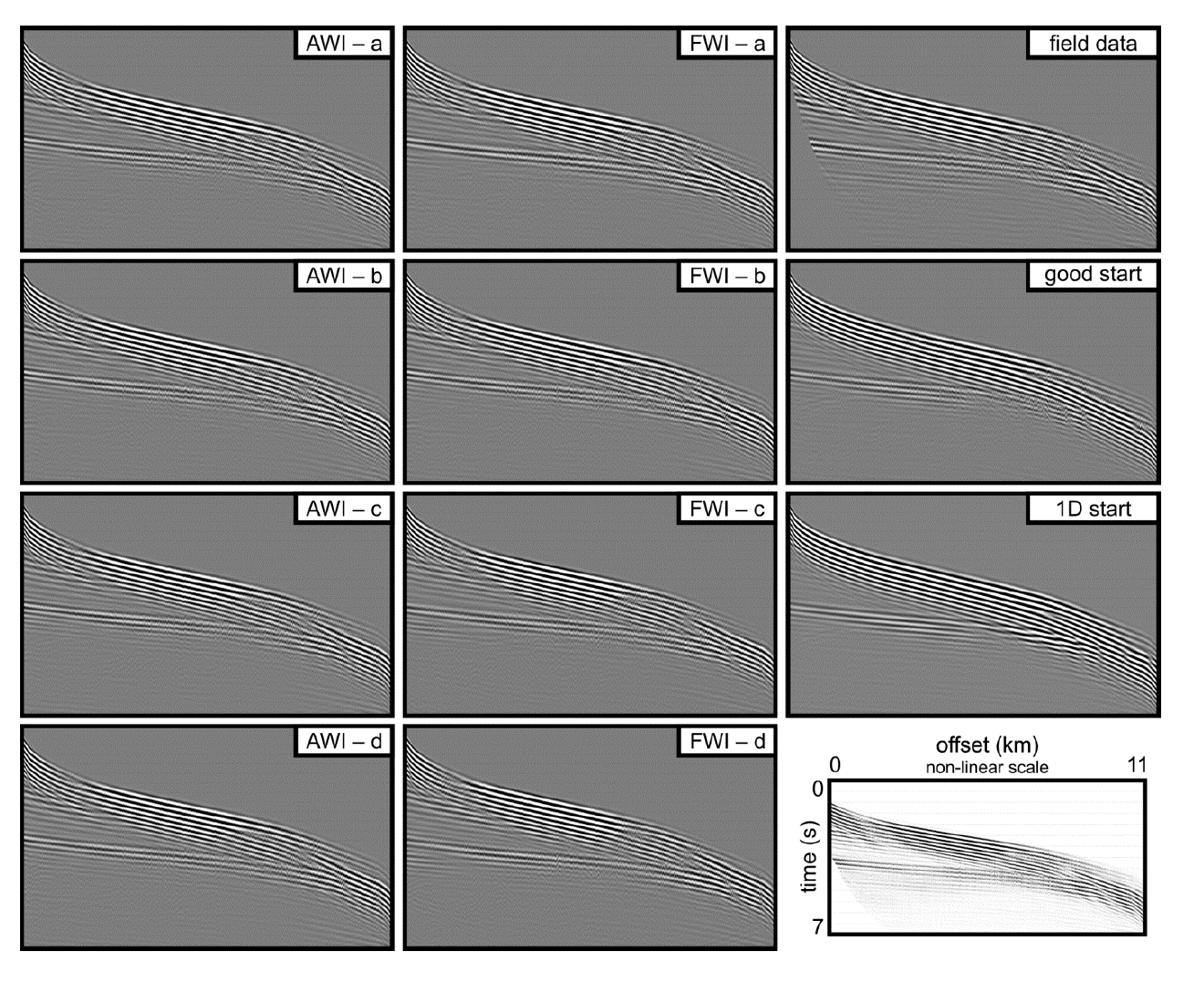
Model validation: predicted and observed data alignment
The panels show different inversion runs for a single randomly selected receiver gather - all offsets. The inversion drives the predicted data towards the observed data.
XWI model evolution
The successful XWITM model evolution employs the AWI objective function for the long to intermediate length scale updates before switching to the FWI objective function for final refinements to the detail.
FWI alone applied from the same starting model and same lowest frequency range leads to waveform inversion misconvergence.

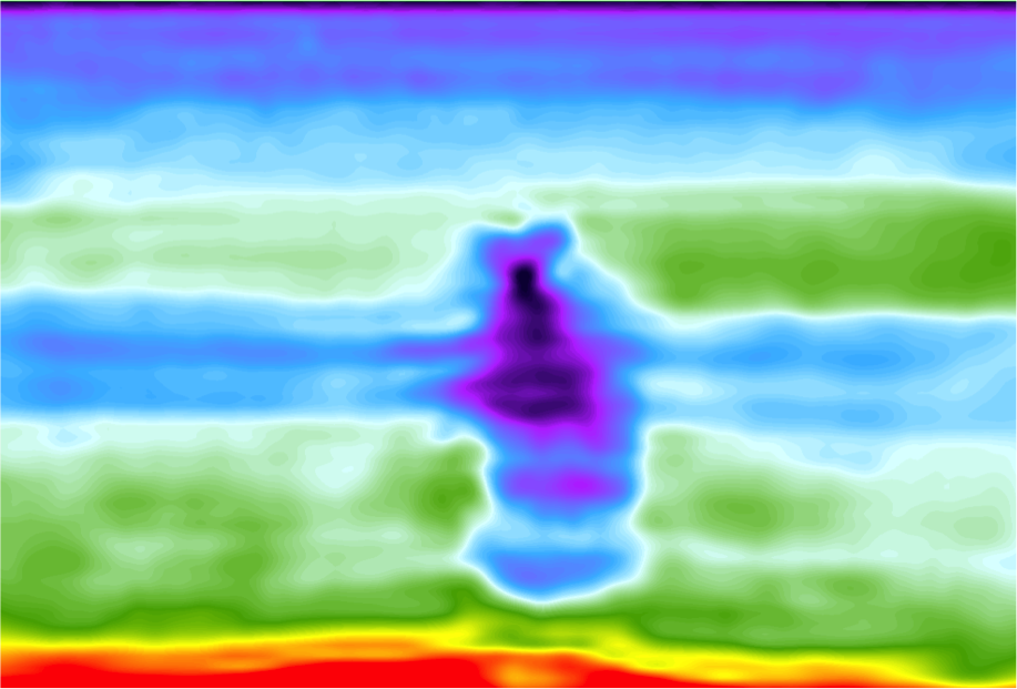
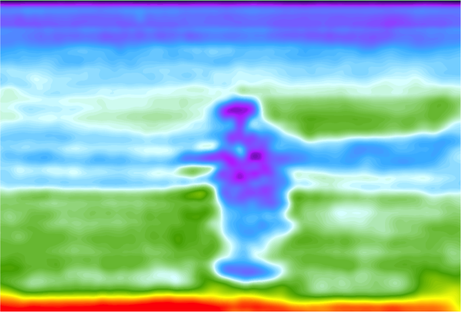
Starting model
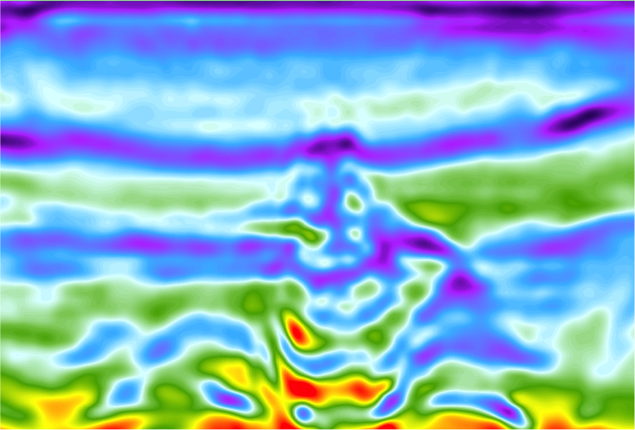
FWI from 1D starting model
Conventional FWI fails due to cycle skipping.
Tomography is required to avoid cycle-skipping and resolve gas cloud...
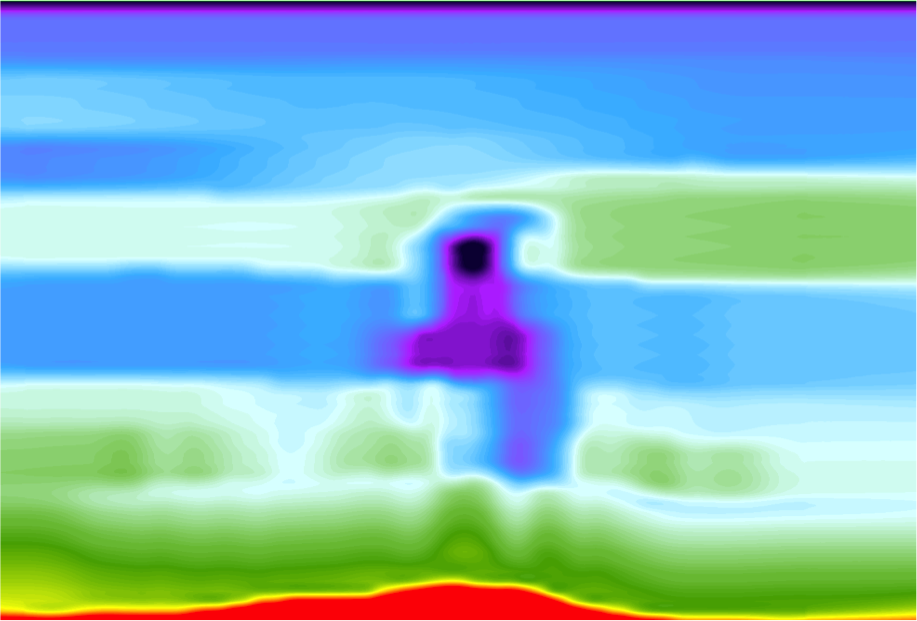
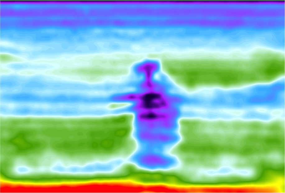
Tomography Model
Tomography then FWI model
However this typically takes 6-12 months.
The Answer?
Cycle Time Reduction with Adaptive Waveform Inversion
AWI converges directly from 1D starting model... No tomography required.
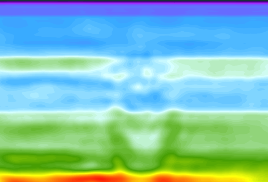
AWI Intermediate Model 1
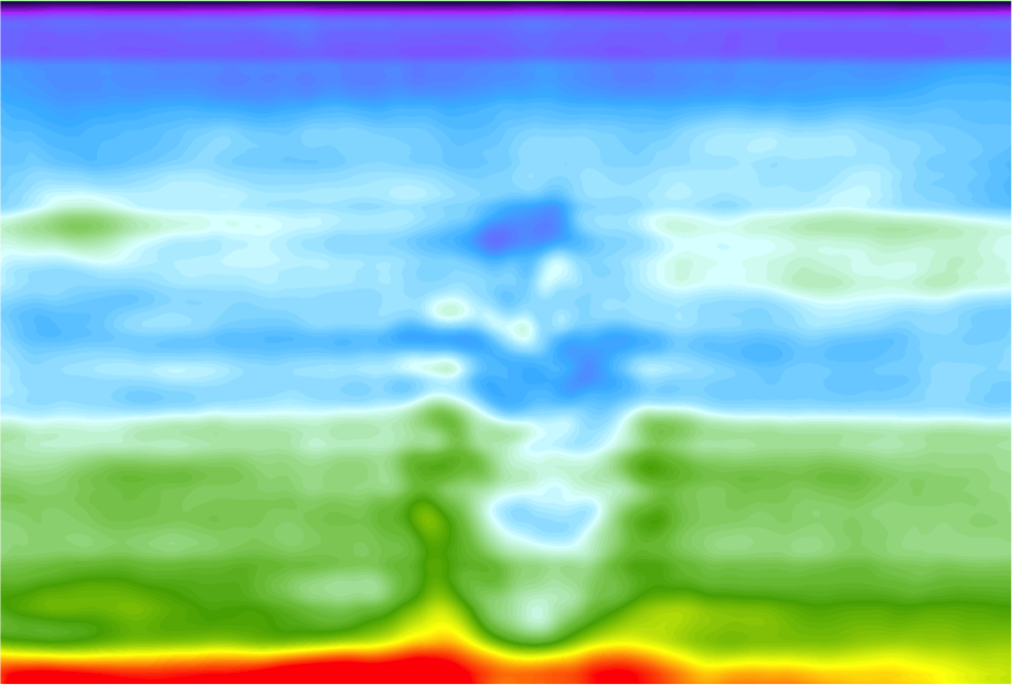
AWI Intermediate Model 2
AWI Intermediate Model 3
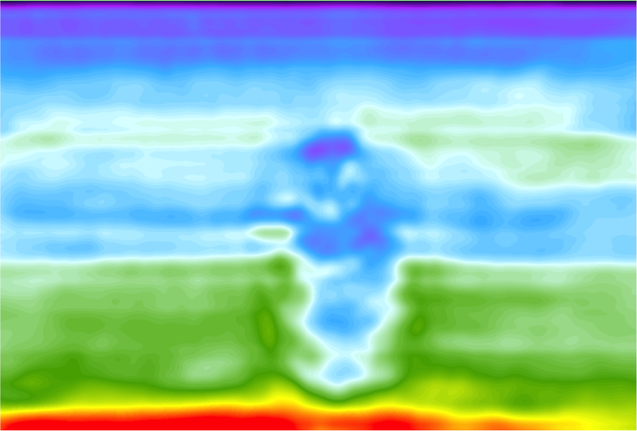
AWI Intermediate Model 4
Final AWI Model starting from a 1D Start